How to add AI to Clinicaltrials.gov

by Josva Engmose Jensen (contact@me-ta.dk)

Posted on December 26, 2018
Updated on January 23, 2019 with predictions using TensorFlow.js

Clinical trials are designed to answer specific questions about biomedical or behavioral interventions in clinical research in the pharmaceutical industry. Clinicaltrials.gov is a huge data base with around 500 new uploaded studies every week from around the world. Whit access to all this data, why not try to feed it into a computer and see if we can do something clever with it? Artificial Intelligence (AI) applications are emerging and performs many tasks in the world we live in today. But how can AI be implemented in simple task in the context of clinical trials? In this paper I will try to walk you trough an example of a rather narrow task, which Deep Learning can help researchers manage clinical trial workflows.

Problem description

The type of task I will guide you through is Supervised Learning, and the data is downloaded from Clinicaltrials.gov. The goal is to predict the type of Interventional model in a study given a summary text and a title from the study. This is a multi-class classification problem, meaning that there is more than two classes to be predicted. After reading this article, you would be able to implement and develop your own LSTM network for your own prediction problems. The process is divided into following steps:

Download trials from link: https://clinicaltrials.gov/AllPublicXML.zip
Reading XML files into .csv files
Reading .csv files into pandas dataframe in python
Pre-process the text data
Modelling and training
Evaluation and prediction

The steps can be described and visualized as:

Import Classes and Functions

I will use a Python3 Anaconda environment together with Jupyter Notebook and i will use Tensorflow backend. Tensorflow is an open source library and it is typically used in machine learning for neural networks.
Here is all the required libraries:

                        
import numpy as np # Linear algebra

# Data processing, CSV file I/O (e.g. pd.read_csv)
import pandas as pd
from pandas import DataFrame

import xml.etree.ElementTree as ET # Reading xml files

# For plotting
import matplotlib.pyplot as plt
import pydot
import pydotplus
import graphviz
from keras.utils.vis_utils import plot_model
from keras.utils import plot_model
from sklearn.manifold import TSNE


# For Modelling
import tensorflow as tf
from tensorflow.keras import layers, models, preprocessing, callbacks, optimizers

print(tf.VERSION)
print(tf.keras.__version__)

from tensorflow.keras.models import Model
from tensorflow.keras.layers import Dense, Embedding, Input, Add
from tensorflow.keras.layers import LSTM, Bidirectional, GlobalMaxPool1D, Dropout
from tensorflow.keras.preprocessing import text, sequence
from tensorflow.keras.callbacks import EarlyStopping, ModelCheckpoint
from tensorflow.keras.optimizers import Adam
from tensorflow.keras.layers import Conv2D, MaxPooling2D, BatchNormalization
from tensorflow.keras.layers import concatenate
from keras.metrics import categorical_accuracy


# For Pre-processing
import string
from string import digits
import nltk
from nltk.corpus import stopwords
from nltk.stem import WordNetLemmatizer
from tqdm import tqdm
import re

# Other useful modules
import h5py
from statistics import mode
import os
import datetime
import warnings
warnings.filterwarnings('ignore')

Download Clinical Trials

The first step is to download all the clinical trials from Clinicaltrials.gov and unpack them into your working directory. After you have done this we are ready to work with the xml files. A good idea would be to investigate the xml files, you can do this in several editors, I personally prefer Visual Studio Code. Get an overview of an xml file and see how it is structured and find the information of your interest.

Working with XML and .csv

XML is an inherently hierarchical data format, and the most natural way to represent it is with a tree. Python has a module for parsing and creating xml data called **xml.etree.ElementTree**. The ElementTree (ET) represents the whole XML document as a tree. We now want to get the contents from our xml files we are interested in. In our case we wish to look at *'nct_id'*, *'brief_summary'*, *'brief_title'* and *'intervention_model'*. The text from these roots are the text that er going into our .csv file. As we have many xml files, we create a function which iterates through the different files and return the text from the 4 different roots. We are not interested in all the xml files, we only look at Phase 2 or 3 and Interventional studies. Here is my code for doing this:

                        
def csv_row(xml_file):

    tree = ET.parse(xml_file)

    root = tree.getroot()

    nct_text = ""
    sum_text = ""
    model_text = ""
    ph_text = ""
    title_text = ""

    # Only iterates through Phase 2 and 3 studies
    for ph in root.iter('phase'):
        ph_text = ph.text
        if (ph_text == "Phase 2" or ph_text == "Phase 3"):

            #This bit finds all roots with nct_id which is a sub_root to id_info
            for nct in root.findall('id_info'):
                nctId_text = nct.find('nct_id').text
                nct_text =nctId_text
                #print(nct_text)

            # This bit finds the brief summary text
            for s in root.findall('brief_summary'):
                summary_text = s.find('textblock').text
                sum_text= summary_text
                sum_text = sum_text.replace('\n', '') # Replaces newline with a whitespace
                sum_text = re.sub(' +',' ',sum_text) # Compresses multiple whitespaces to only one
                #print("Summary Text:", sum_text)

            # Get's the official title for the study
            for t in root.iter('brief_title'):
                title_text = t.text

            # This get's the type of intervention_model
            for y in root.iter('intervention_model'):
                model_text = y.text

    total_text = "\"" + nct_text + "\"" + ";" + "\"" + sum_text + "\"" + ";"  + "\"" + title_text + "\"" + ";"  +  "\"" + model_text + "\""

    # This functions returns a text with Nct_Id, brief_summary, title and type of intervention model on the form we intended

    return total_text

    csv_row("search_result\\NCT00496392.xml")# This is for checking that the function works

We now have a function that returns the text of interest and the text is seperated with ';', which is one of standard seperators in .csv files. As you can see from this text, it contains symbols, which we are not interested in when training our model, but more about that later :) We now wish to write this text into 2 different .csv files, which is showned below:

                        
rdir = 'Subset_data' # Folders in directory where the all the xml files are placed

    with open('train_data.csv', 'w', encoding="utf-8") as csvfile: # Opens a blank csv file
        with open('test_data.csv', 'w', encoding="utf-8") as csvfile1:
            for _, dirs, _ in os.walk(rdir):
                for dir in dirs: # Looks at  all the xml folders
                    if dir < 'NCT0012': #This is around 80% of the folders
                        for subdir, _, files in os.walk(os.path.join(rdir,dir)):
                            for file in files:
                                name = os.path.join(subdir, file)
                                csvfile.write(csv_row(name)) #Writes total_text into a row in to train_data.csv
                                csvfile.write("\n") # Skips to next line and do the same
                    else: #This is the remaining 20% of the folders
                        for subdir, _, files in os.walk(os.path.join(rdir,dir)):
                            for file in files:
                                name = os.path.join(subdir, file)
                                csvfile1.write(csv_row(name)) #Writes total_text into a row in to test_data.csv
                                csvfile1.write("\n")

As you can see from my code above, we condition on the size of string in foldernames to make an appropriate division of train and test data. It is approximately about 80% training data and 20% test data. Another approach for this could be loading the data into a pandas dataframe and use the function train_test_split from the sklearn module, and here you should specify the test_size. 80/20 split is very common in machine learning algorithms *(Bronshtein, A. 2017, Train/Test Split and Cross Validation in Python. [https://towardsdatascience.com/train-test-split-and-cross-validation-in-python-80b61beca4b6])*.
We now have 2 .csv files with containing the data of our interest.

Reading into Pandas

We now wish to read our 2 .csv files into dataframes in python, and here we can use the module called pandas. The pandas module has a simple function doing this: **pd_read_csv**, and here is how you use it:

                        
# Earlier we saw that the returned text from our function was seperated by ';', so we use this as seperator when reading in the files
tr_df = pd.read_csv("train_data.csv", sep=';', header=None,error_bad_lines=False, warn_bad_lines=False)
t_df = pd.read_csv("test_data.csv", sep=';', header=None,error_bad_lines=False, warn_bad_lines=False)

# Give the data sets appropiate column names
tr_df.columns =  ['Nct_id', 'Summary', 'Title',"Model"]
t_df.columns =  ['Nct_id', 'Summary', 'Title',"Model"]

# We drop all the observations containing NaN's (missing values)
train = tr_df.dropna()
test = t_df.dropna()

This now gives us 2 dataframes with rows and columns corresponding to our .csv files. As you can see in my code i have specified the column names myself. It is now a good idea to visualize your response variable and plot the distribution. In our case it is a categorical variable, so this will be a bar plot. In the figure below I have plotted the different types of models from a small subset of our data and the belonging code is also specified.

                        
import seaborn as sns
sns.set(style="darkgrid")
ax1 = sns.countplot(x="Model", data=train, order = train['Model'].value_counts().index)
ax1.set_title("Barplot for types of Intervention models")
for item in ax1.get_xticklabels():
    item.set_rotation(45)

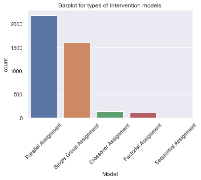
Barplot for types of intervention models

As you can see in the plot there are many Parrallel and Single Group study designs compared to the others. This is only a small subset of the data from Clinicaltrials.gov, so we can still be able to train a computer to predict the other categories. However we are not interested in Factorial or Sequential Assignment, so we will collect this into one category we call 'Other'. This means that our response variable now can take 4 different values.

Some Machine Learning algorithms supports categorical values, but there are many cases where the algorithms does not. The data analyst is therefore faced the challenge of turning these text attributes into numerical values for further processing. There are many different ways of encoding categorical variables, but one approach could be 'Label Encoding'. This is simply converting the different values in our response to a number. This is easily done in python:

                        
# We want 4 categories: Crossover, Parallel, Single Group and Other
train.loc[(train['Model'] == 'Factorial Assignment'), 'Model'] = 'Other'
train.loc[(train['Model'] == 'Sequential Assignment'), 'Model'] = 'Other'
test.loc[(test['Model'] == 'Factorial Assignment'), 'Model'] = 'Other'
test.loc[(test['Model'] == 'Sequential Assignment'), 'Model'] = 'Other'

# Convert from object to category
train['Model'] = train['Model'].astype('category')
test['Model'] = test['Model'].astype('category')

#Label encoding
train["Model_type"] = train["Model"].cat.codes
test["Model_type"] = test["Model"].cat.codes
train.head() # Prints the first 5 rows of the data

The index in the left side of the dataframe just corresponds to the rows from the .csv file. By default python will encode the categorical values by alphabetic order, so it will be encoded as:

0: Crossover Assignment
1: Other
2: Parallel Assignment
3: Single Group Assignment

Label Encoding as you can see is straightforward and easily implemented, but it has the disadvantage that the numeric values can be “misinterpreted” by the algorithms. The value 3 is obviously larger than the value 1, but the category *'Single Group Assignment'* is not larger than *'Crossover Assignment'*. This is the case whenever your categorical variable is nominal, which means that there is no natural ordering between the categories.

Another common approach is called one hot encoding *(Francois Chollet, 2018. Deep Learning with Python. Manning Publications Co., Shelter Island, NY, 361 pp. )*. The basic idea is to convert each category into a new column as a dummy variable (0/1). This will not weight the values as in label encoding, but it does add more columns to the data set. Pandas has a feature which support this:

                        
# One Hot Encoding
train_dummy = pd.get_dummies(train, columns=['Model'], prefix =['Model'])
test_dummy = pd.get_dummies(test, columns=['Model'], prefix =['Model'])
print("Train shape:",train_dummy.shape)
print("Test shape:",test_dummy.shape)

I suggest, as i do in my code, to print the shape of the data sets or maybe print the first 5 rows to verify. Before we only had 4 columns and now we have 8, where the last 4 corresponds to the dummy variable for each of the categories. In our case we only have these 4 mentioned categories, but it can be challenging to manage this is, if you have a large amount of categories.

Text Preprocessing

When dealing with textual data, it needs to be cleaned and encoded to numerical values before feeding them into machine learning models, this process of cleaning and encoding is called Text Preprocessing.

I will perform basic cleaning steps on the two features 'Title' and 'Summary', so it will be ready to be fed into a classifier. *(Siddiqi, S. 2018, Text Preprocessing for Beginners - Data Cleaning. [https://www.kaggle.com/sabasiddiqi/workbook-1-text-pre-processing-for-beginners])*

The following steps will be performed:

Removal of punctuation
Removal of newline symbols (\n)
Removal of digits
Splitting combined words
Converting words to lowercase
Splitting each sentence using delimiter
Converting words to base form

Here is my code for the above pre-processing steps:

                        
# This needs to be download for the lemmatization (converting to base form)
nltk.download("wordnet")

                        
def text_cleaner(dataframe_org):
    dataframe = dataframe_org.copy()

    columns = ['Summary', 'Title']

    for col in columns:
        dataframe[col] = dataframe[col].str.translate(str.maketrans(' ', ' ', string.punctuation)) # Remove punctuation
        dataframe[col] = dataframe[col].str.translate(str.maketrans(' ', ' ', '\n')) # Remove newlines
        dataframe[col] =dataframe[col].str.translate(str.maketrans(' ', ' ', digits)) # Remove digits
        dataframe[col] =dataframe[col].apply(lambda tweet: re.sub(r'([a-z])([A-Z])',r'\1 \2',tweet)) # Split combined words
        dataframe[col] =dataframe[col].str.lower() # Convert to lowercase
        dataframe[col] =dataframe[col].str.split() # Split each sentence using delimiter

    # This part is for converting to base form
    lemmatizer = WordNetLemmatizer()
    sum_l=[]
    tit_l = []
    for y in tqdm(dataframe[columns[0]]): # tqdm is just a progress bar, an this loop only looks at summaries
        sum_new=[]
        for x in y: # Looks at words in every summary text
            z=lemmatizer.lemmatize(x)
            z=lemmatizer.lemmatize(z,'v') # The v specifies that it is in doubt of example a word is a noun or verb, it would consider it a verb.
            sum_new.append(z)
        y = sum_new
        sum_l.append(y)
    for w in tqdm(dataframe[columns[1]]): # Looks at titles
        tit_new=[]
        for x in w: # Every word in the titles
            z=lemmatizer.lemmatize(x)
            z=lemmatizer.lemmatize(z,'v')
            tit_new.append(z)
        w = tit_new
        tit_l.append(w)

    # This will join the words into strings as in the original data, just pre-processed and put into list
    sum_l2 = []
    for col in sum_l:
        col = ' '.join(col)
        sum_l2.append(col)
    tit_l2 = []
    for col in tit_l:
        col = ' '.join(col)
        tit_l2.append(col)

    # Data obtained after Lemmatization is in array form, and is converted to Dataframe in the next step.
    sum_data=pd.DataFrame(np.array(sum_l2), index=dataframe.index,columns={columns[0]})
    tit_data=pd.DataFrame(np.array(tit_l2), index=dataframe.index,columns={columns[1]})

    frames = [sum_data, tit_data]
    merged = pd.concat(frames, axis=1)
    return merged


def create_tok(train_data, MAX_FEATURES):
    clean_data = text_cleaner(train_data)

    tokenizer_sum = text.Tokenizer(num_words=MAX_FEATURES) # Keep the 20.000 most frequent words
    tokenizer_tit =  text.Tokenizer(num_words=MAX_FEATURES)

    # Summary Text
    summary_list = clean_data['Summary']
    tokenizer_sum.fit_on_texts(list(summary_list)) # Builds the word index

    #Title Text
    title_list = clean_data['Title'] # Text from Title
    tokenizer_tit.fit_on_texts(list(title_list))

    return tokenizer_sum, tokenizer_tit

def pre_process(dataframe, tokenizer, col, MAXLEN):
    clean_data = text_cleaner(dataframe)
    tokenized_list = tokenizer.texts_to_sequences(clean_data[col])
    X = sequence.pad_sequences(tokenized_list, maxlen=MAXLEN)

    return X

I will now try to explain some of the above code, besides the comments i have made in transit.

We need to keep in mind that deep learning models does not truly understand text in human sense, but they can be great for solving simple textual tasks. Like all neural networks, deep learning models can't be fed with raw text as input, text data must be encoded as numbers. Keras provides the Tokenizer class for preparing text for deep learning *(Francois Chollet, 2018. Deep Learning with Python. Manning Publications Co., Shelter Island, NY, 361 pp. )*. This Tokenizer is fitted on the text data as you can see in my code.

The text.Tokenizer() is chopping the sequences of text into sequences of **'tokens'**, where these tokens represents the meaning of the words in a dictionary. The **'tokenized_list'** will now be a list of lists containing only integers representing the words, and the **'X'** will be a list of lists.

The .pad_sequences() is used to ensure that all sequences in a list has the same length. This is done by padding 0's in the beginning of each sequence until each sequence has the same length as the longest sequence. So if the sequence for example has length 200, the first 100 elements will be filled with 0's.

We can now run this function on our train and test data sets:

                        
MAX_FEATURES = 20000 # Size of vocabluary
MAXLEN = 300 # Size of each text sequence, you can tune this depending on the mean length of you text sequences

tok_sum, tok_tit = create_tok(train_dummy,MAX_FEATURES )

# The following are used for model.fit
X_sum = pre_process(train_dummy, tok_sum, 'Summary', MAXLEN)
X_tit = pre_process(train_dummy, tok_tit, 'Title', MAXLEN)

# This is used for prediction
X_sum_test = pre_process(test_dummy, tok_sum, 'Summary', MAXLEN)
X_tit_test = pre_process(test_dummy, tok_tit, 'Title', MAXLEN)

list_classes = ["Model_Crossover Assignment", "Model_Other", "Model_Parallel Assignment", "Model_Single Group Assignment"] # The 4 categories
y = train_dummy[list_classes].values

# y_test is used for model.evaluate later on
y_test = test_dummy[list_classes].values

We now have every thing we need to train a deep recurrent neural network. But before doing that I will just take some time and briefly explain something about LSTM network.

Long short-term memory

The Long Short-Term Memory network or LSTM network is a type of recurrent neural network used in deep learning. It was developed becuase of the lack of RNN, and LSTM can solve the problem long-term dependency, beacuse it uses gates to control the memorizing process.

LSTM is typically used for language modeling, sentiment analysis and text prediction. It has the ability to forget, remember and update information, and this pushes it one step ahead of RNN's. If you want to perform Supervised Learning with sequences as input, you want to use a gated recurrent net such as LSTM or GRU. If your input is for example images or of other topological structure the best approach would be a convolutional network. *(Goodfellow, I. and Bengio, Y. and Courville, A. 2016. Deep Learning. MIT Press. 781 pp. [https://www.deeplearningbook.org/] )*

Below you see a figure that visualize how an LSTM network is structured.

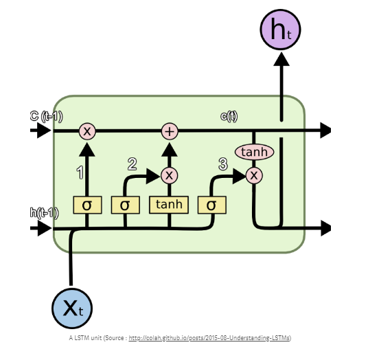
I will now try to breifly explain the figure.

There are 3 main components of LSTM units:

1. It can forget unnecessary information. A Sigmoid layer, which outputs a number between 0 and 1 is used to forget or remember information. It looks at the current input (Xt) and the previous output (h(t-1)), and decides which part of the previous output there should be removed (if the sigmoid returns a 0). This we call the forget gate, f(t), where the output is f(t) * c(t-1), where c(t-1) is the memory from the last LSTM unit.
2. Then it needs to decide which information to store from the new input X(t). Sigmoid decides if the information should be updated or ignored, and a tanh layer creates a vector of values for new input. If these 2 are muliplied, it will update the new cell state. The new memory from these 2 layers are added to the old memory (c(t-1)) to give us c(t).
3. The last step is to decide what the output should be. A sigmoid layer decides which parts from the cell state (c(t)) we will output. Then the cell state is put through a tanh, which will generate all possible values and is mulitplied with the output from the sigmoid gate. So the output is only the parts we decide to output.

So in a few words a LSTM model will not learn from the immediate dependency, it will learn from long term dependency. *(Sinha, M. 2018. Understanding LSTM and its quick implementation in Keras for sentiment analysis. [https://towardsdatascience.com/understanding-lstm-and-its-quick-implementation-in-keras-for-sentiment-analysis-af410fd85b47])*

Building a model

Now we have a little idea of what a LSTM network is and we will now try to build one.

My code for this is showned below, and I will try to explain it afterwards.

                        
def get_con_model():
    embed_size = 50 # How big  each word vector should be

    inp_sum = Input(shape=(MAXLEN, ))
    inp_title = Input(shape=(MAXLEN, ))

    total_inp = concatenate([inp_sum, inp_title]) # Merge the 2 inputs

    embed_layer = Embedding(MAX_FEATURES, embed_size)(total_inp)
    lstm_layer = LSTM(50)(embed_layer)
    layer1 = Dropout(0.1)(lstm_layer) # Regularization method, has the effect of reducing overfitting
    layer2 = Dense(50, activation="relu")(layer1) # The relu function can return very large values
    layer3 =  Dropout(0.1)(layer2) # Again regularization
    layer4 =BatchNormalization()(layer3) # Maintains the mean activation close to 0 and the activation standard deviation close to 1
    layer5 = Dense(4, activation="softmax")(layer4) # Only outputs values between 0 and 1, this is the final layer

    model_con = Model(inputs=[inp_sum,inp_title], outputs=layer5)
    model_con.compile(loss='categorical_crossentropy', # This is the loss function, and this type of function is used when solving categorical classification
                    optimizer='rmsprop', # Algorithm that update network weights iterative based in training data
                    metrics=['accuracy']) # This is our statistical measure

    return model_con

con_model = get_con_model()

# Gets informations about the layers in the model, including output, input and number of parameters:
con_model.summary()

I suggest to always look at the summary and to visualize your model. Here are some few reasons to that:

**To confirm the layer order**. It is easy to make mistakes and adding layer in the wrong order, and the plot of the model can help you confirm that it is done right.

**To confirm parameters**. Number of parameters are given in the model.summary, and it can help you spot possible layers to reduce number of parameters.

**To confirm the output shape of the layers**. In complex networks it can be difficult to specify the shape of input data. The summary and the plot can help you confirm the shapes as you intended.

We will now visualize our network, and to do so you need to make sure you have Graphviz installed separately on your system, not just in your project directory. It can be downloaded from https://www.graphviz.org/download/.
Here is the code for plotting our model:

                        
                            os.environ["PATH"] += os.pathsep + 'C:/Program Files (x86)/release/bin/'
                            plot_model(con_model, to_file='model_plot.png', show_shapes=True, show_layer_names=True)

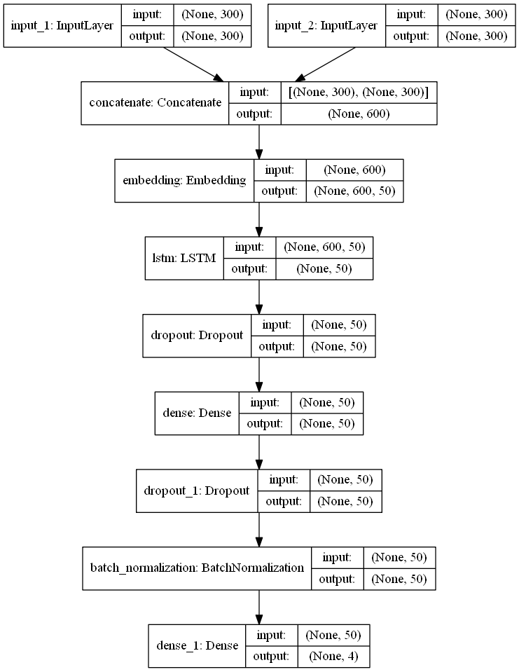
If we walk through the steps, we see the first thing is the 2 input layers, and we do not differ between MAXLEN (input) for summary and title text, for simplicity. Next we concatenate the 2 input layers before embedding, and this is primarily done to reduce the number of parameters in the model, because number of parameters from an embedding layer is **MAX_FEATURES** times **embed_size**, which in this case is 1 million parameters. Then comes the Embedding layer, which takes the concanated input layer as input. The meaning of word embedding is to map human language into a geometric space. In this space we would like synonyms to be embedded into similar word vectos, and that the geometric distance between 2 word vectors would relate to the semantic distance. The word representation with word embedding become relatively low dimensional and dense, beacuse it is learned from data. This is a clear benefit compared to one-hot word vectors, which is high dimensional and hardcoded. *(Francois Chollet, 2018. Deep Learning with Python. Manning Publications Co., Shelter Island, NY, 361 pp. )*
For word embedding to make a little bit more sense, i will now try to visualize it:

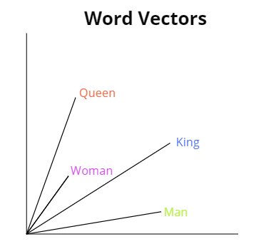
In the figure above, we have 4 words embedded in 2D: *Man*, *King*, *Woman* and *Queen*. With vector representations, the semantic relationships between the words can be encoded as geometric transformations. In this case the same vector allows us to go from *Man* to *King* and from *Woman* to *Queen*. We could interpret this vector as *"From gender to royal status"*. In the same way we could also consider the vector which allows us to go from *King* to *Queen* and from *Man* to *Woman*.
The type of word embedding depends on your problem, and you have to consider in which context it is used. Their exists some pretrained embedding files on the internet, which may can be useful for your task (Fx GloVe). We chosed to use the embedding layer from the keras.layers.
The next layer in our network is an LSTM layer, where the output from the **embed_layer** is given is input. Here the number of LSTM units is set to 50, which is the dimensionality of the output space of this layer. After the LSTM layer we have a Dropout layer. Dropout is a common regularization technique *(Francois Chollet, 2018. Deep Learning with Python. Manning Publications Co., Shelter Island, NY, 361 pp. )*, which randomly select neurons that are ignored during the training and the weight updates are not applied to the neuron. The dropout rate, which in this case is set to 0.1, corresponding to 10%. You can tune this hyperparamter while experimenting building your own model.
After the first dropout layer we have a Dense layer, which is just a regular layer of neurons in a neural network. Each neuron recieves input from all the neurons in the previous layer, thus densely connected. In this layer we used the activation function **'relu'** which range is from (0,inf), and with this function we can pass the maximum of the error through the network. A result of this layer could be very large outputs, which the network finds very challenging to handle. We use again a dropout layer, with the same 10% dropoutrate. The next layer is **BatchNormalization** which is a way of mantain the mean activation to be close to 0 and the standard deviation to be close to 1, this handles the possible large outputs from the dense layer with our relu function *(Keras Documentation, [https://keras.io/layers/normalization/])*. Our final layer uses **softmax** as activation function, and this function only outputs probabilities range. The range is therefor from 0 to 1 and the sum of all the probabilities will be equal to one. The reason why we set units in the Dense layer to 4, is that we have 4 catogories, and the model returns probabilities for each of these categories, where the target has the highest probability.
Before we train our model, there is a few parameters we should specify. We need to give the model.fit a **batch_size**, which is the number of samples that will be propagated through the network. We have set this to 32, which means that the algorithm will take the first 32 samples and train the network. Next it takes the second 32 samples and trains the network again. We continue with this process until we have propagated all samples in our data through the network.
A benefit of using af batch size smaller than the number of samples, is that it requiers less memory. This can be very profitable when having a large data set. Our network will also train faster. The reason for this is that we update the network parameters after each propagation, but if we used all the samples it will only update 1 time *(2015. What is batch size in neural network?, [https://stats.stackexchange.com/questions/153531/what-is-batch-size-in-neural-network] )*.
We also need to specify something called **epoch**. An epoch is simply the number of passes over the entire data set. This number can vary a lot, but for a start we will set it to 10 and later on we will set it lower, but more about that in a minute. In our case we have 3625 samples and since we chosed our batch size to be 32, it will take 3625/32 = 114 iterations to complete one epoch.
We will now train our model and i will explain rest of the code below after the training.

                        
batch_size = 32 # number of samples that will be propagated through the network.
epochs = 10 # Number of passes over the entire data set

file_path="weights_base.hdf5"

checkpoint = ModelCheckpoint(file_path, monitor='val_loss', verbose=1, save_best_only=True, mode='min') # Verbose means that it prints acc and loss
early = EarlyStopping(monitor="val_loss", mode="min", patience=3) # EarlyStopping should only be includede when tuning your model

callbacks_list = [checkpoint, early]

history = con_model.fit([X_sum, X_tit], y, batch_size=batch_size, epochs=epochs, validation_split=0.1, callbacks=callbacks_list, verbose=2) # Model fit

You can safely ignore the warning. It's a preemptive warning from TensorFlow when it cannot be certain of the size of the generated tensor
The model has now trained on our training data, and i will now explain what is actually writtin in my code and why i have done it the way i did.
A common problem in Machine learning algorithms is the term called overfitting. If we train our model we will see that the training loss decreases with every epoch and the training accuracy increases. A model that performs better on training data will not necessarily be a model that will do better on completely new data. A way of preventing your model to overfit, we have made someting called a validation split. *(Brownlee, J. 2016. Overfitting and Underfitting With Machine Learning Algorithms. [https://machinelearningmastery.com/overfitting-and-underfitting-with-machine-learning-algorithms/])*
In this split we will save 10% of our training data as validation. As you can see in my code, i have made the validation split in the model.fit and specified an early stopping. The early stopping is set to avoid keep training the model when we don't see an improvement in validation loss. Sometimes local minima can occur, and this is why you give early stopping some patience, and in our code we set it to 3, which means if we don't see an improvement 3 epochs in a row, the model will stop training.
We now visualize the model accuracy and loss from our training:

                        
# Final evaluation of the model
%matplotlib inline
plt.plot(history.history['acc'])
plt.plot(history.history['val_acc'])
plt.title('model accuracy')
plt.ylabel('accuracy')
plt.xlabel('epoch')
plt.legend(['train','val'], loc='upper left')
plt.show()

%matplotlib inline
plt.plot(history.history['loss'])
plt.plot(history.history['val_loss'])
plt.title('model loss')
plt.ylabel('loss')
plt.xlabel('epoch')
plt.legend(['train','val'], loc='upper left')
plt.show()

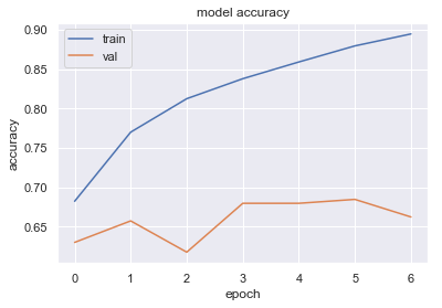
From the above plots we set the number of epochs to 4 and remove the early stopping and validation split and now use all of the training data in our training.

                        
batch_size = 32
epochs = 4

file_path="weights_base.hdf5"
checkpoint = ModelCheckpoint(file_path, monitor='loss', save_best_only=True, mode='min')

                        
history = con_model.fit([X_sum, X_tit], y, batch_size=batch_size, epochs=epochs, callbacks=[checkpoint], verbose=2)

                        
Epoch 1/4
- 48s - loss: 0.9551 - acc: 0.6696
Epoch 2/4
- 44s - loss: 0.6527 - acc: 0.7686
Epoch 3/4
- 44s - loss: 0.5618 - acc: 0.7972
Epoch 4/4
- 51s - loss: 0.4942 - acc: 0.8222

We see that this gives us an accuracy of around 82%, but let's evaluate the model and see how good it is to handle completely new data (test data)

                        
con_model.load_weights(file_path)
con_model.evaluate([X_sum_test, X_tit_test], y_test, verbose=2) # Returns loss value and the metric specified, so in this case, model accuracy

[0.7706552325145077, 0.7159199235096105]

We now get an accuracy of almost 72 %, and this is not a bad result at all. We have only trained the model on a small subset of the total data set (only 4000 studies) and it seems that the model is doing quite okay, and we can generalize it to complete untrained data.

Prediction

We have now trained and evaluated our LSTM network. But to get a feeling about how it actually works and to demonstrate how it can be used for new clinical trials i will now give some examples of some new data and make prediction from that.
In my code below i have made a function which takes a Title and a Summary and put into a pandas dataframe. This data is going through the same pre-processing as our train and data set, so it is ready to be fed into our model.

                        
def my_pred(Title, Summary):

original_data = pd.DataFrame({ 'Summary' : [Summary],
'Title': [Title]})

# Clean data
X_pred_sum = pre_process(original_data, tok_sum, 'Summary', MAXLEN)
X_pred_tit = pre_process(original_data, tok_tit, 'Title', MAXLEN)

con_model.load_weights(file_path)
prediction = con_model.predict([X_pred_sum, X_pred_tit])

return prediction

We have taking a study, which is not a part of our train data and we will now try to predict the type of intervention model from the summary text and title. First as you see below we try where we specify the full summary text and all of the title:

                        
Study_sum = "This clinical trial will be performed in previously untreated patients with metastatic
colorectal cancer. The study will evaluate the safety, tolerability and efficacy of the study drug,
CT-011, in combination with FOLFOX chemotherapy (FOLFOX4 or mFOLFOX6) compared with treatment by
FOLFOX alone."
Study_tit = "Study to Evaluate the Safety, Tolerability and Efficacy of FOLFOX + CT-011 Versus
FOLFOX Alone"
my_pred(Study_tit, Study_sum)

array([[0.01352272, 0.01536347, 0.8943102 , 0.07680359]], dtype=float32)
We get a prediction of 89%, that this study is a Parallel Assignment and this is also the case. But what if we can just use the title as predictor and give the model an empty summary? Let's look at that!

array([[0.01352273, 0.01536347, 0.8943102 , 0.07680362]], dtype=float32)
In this case we get accurat the same prediction as with the full summary text. The title is almost always a short and compact version of the summary, so it contains many of the same words, which our model most likely find interesting. It therefor make great sense, that the prediction is identical. Let's now try to give the model some few key words from the title and still let the summary text be empty and see what happens.

                        
key_tit="Study Evaluate Safety, Tolerability Versus Alone"
my_pred(key_tit, empty_sum)

array([[0.01274031, 0.01423935, 0.8709181 , 0.10210223]], dtype=float32)
We see that our model now predicts 87%, so just a little bit lower than before. So whether the model predicts what type of model it is, depends only on some few key words, and it is still accurate without being specific in the title our summary if the study is for example Parallel or Crossover.

Summary

In this article you have learned how to build a LSTM recurrent neural network for categorical prediction in Python and using Tensorflow (Keras) deep learning network.
Specifically important things:

Prepraring textual data to feed into a neural network
How LSTM can be useful in the context of clinical trials
How to create an LSTM network for categorical prediction
How to evaluate a model
Make predictions from a model

Article as pdf

Finnaly, let's try it out!

Below you will see two textboxes which i have already been filling out with information from a random study, in this case a Parallel Assignment, from clinicaltrials.gov.
To get the predictions, just click on the "Get Prediction" button and 4 probabilties will now appear in the table. You can just erase my text and try with your own study.

Thanks for reading! Enjoy!

Put your text here:

Summary:

Title:

Your Predictions:

Crossover Assignment	Other Assignment	Parallel Assignment	Single Group Assignment

Interested to learn how you come from building a model to implementation on a web site?
Read this article.